Trading using Technical Indicators on Blueshift®¶

What are technical indicators¶

Technical indicators are, in general, functions of price and volume of underlying securities¹. There are many indicators - essentially differing in their functional forms. However, most indicators can usually be expressed as a function of returns of the underlying. For example, the moving average cross-over indicator is the difference in two different moving averages of price. This can be expressed as $mom=\sum_{i=0}^{n_1} a_i.P_i - \sum_{i=0}^{n_2} b_i.P_i$ where $n_1$ and $n_2$ are the short and long moving average periods, $a_i$ and $b_i$ are weights for the price points (for simple moving averages $a_i=1/n_1$ etc.) and $P_i$ s are the price points. It can be shown² that this can be expressed in terms of price returns, as $mom=\sum_{i=0}^{n} w_i.r_i$ , where $r_i=P_i - P_{i-1}$ and $n=n_2$ from above. The $r_i$ s are returns, if we assume $P_i$ s are log prices. Similar treatment can be applied to other indicators, a few examples below

Momentum cross-over: $\sum_{i=0}^{n} w_i.r_i$
MACD histogram (MACD line - signal line): $\sum_{i=0}^{n1} w_i^1.r_i - \sum_{i=0}^{n2} w_i^2.r_i\Rightarrow\sum_{i=0}^{n} w_i.\Delta{r_i}$ , here $\Delta{r_i}=r_i - r_{i-1}$
CCI: $\frac{1}{\sigma}\sum (P_i - \bar P)\Rightarrow\frac{1}{n.\sigma}\sum (r^{n}+r^{n-1}+..+r)\Rightarrow\sum w_i.r_i$ where $r^k = r_i - r_{i-k}$

Nature of technical indicators¶

While most indicators can be expressed as a function of returns, not all of them are linear (or even polynomial) as above. Broadly, we can divide all common technical indicators that can be expressed as function of returns in three different classes:

Indicators that are linear (or polynomial) combination of past returns in returns space ( $f(r)$ ). Examples - the ones above. Under certain condition (stationarity) they can be modeled as Gaussian distribution
Indicators that are functions of sign of the returns in signed returns space ( $f(r^+, r^-)$ ). Examples - like RSI or Chande Momentum Oscillator. They can be analyzed using folded normal distribution
Indicators that are function of returns in time space ( $f(t(r))$ ). An examples is the Aroon indicator.

Different indicators may have significant commonalities - given they all are essentially filters over the prices (and volumes). However, the response characteristics of their filtering method may differ, based on the functional form, as well as the parameters used (e.g. lookback etc). MACD, for example is more mean-reverting (i.e. suitable for short term trends) compared to momentum cross-over with similar parameters. Also increasing the lookback periodicity for most indicators will make them less sensitive to short term fluctuations.

A simple strategy¶

Let's implement a simple technical indicators based strategy on Blueshift®. It is based on simple moving averages and bollinger band.

bbands

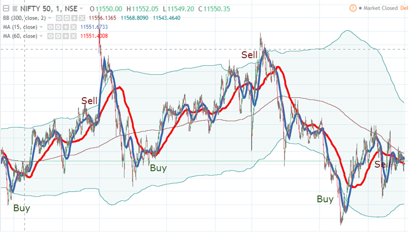
We buy (sell) if the close price is near lower (upper) bands. If price is away from either extreme we buy (sell) if momentum cross-over is positive (i.e. short term moving average is higher than long term one).

Implementing technical indicators¶

On Blueshift®, the easiest way to implement any common technical indicator is using the talib library. This is a Python wrapper for the c-library TA-lib.

Note

Most of the functions in talib will accept a single (or multiple) numpy array as inputs. The data functions on Blueshift® will usually return a Pandas series or dataframe. To use the data, use the values attribute of Pandas object to access the underlying numpy array.

The basic code snippet looks like below:

# import talib
import talib as ta

# inside some functions like handle data
px = data.history(symbol("AAPL"), "close", 100, "1d")
upper, mid, lower = ta.BBANDS(px.values)

Creating our own technical indicator library!¶

If we plan to use technical indicators heavily in our strategy code, it perhaps make sense to create a re-usable library in our workspace. Create a directory at the top level of your workspace named library (if it is not already there). Inside that directory, create another directory named technicals (of not there already). Create a source file named indicators, using any template, under the directory technicals. Click the source to open in the code editor and delete the existing code. Copy the content of from here and paste it in the code editor. Save and go back to workspace root. Now we have a library with a useful bunch of technical indicators ready to be used in our code anywhere with a single line of code

from blueshift_library.technicals.indicators import macd

Creating the strategy¶

Now we get our hands dirty to code the strategy. Create a source file anywhere in your workspace, using the Buy and Hold (NSE) template. Open it in code editor (by clicking it). This template already includes most of the import we required. Let's add an import statement at the very top to include our own technical indicator library we just created. We also import commission and slippage to set them to zero in our demo strategy.

from blueshift_library.technicals.indicators import bollinger_band, ema
from blueshift.finance import commission, slippage

Let's now delete everything from the initialize function in the template and below.

Defining the `initialize` function¶

Now let's overwrite the initalize function to look like below

def initialize(context):
    # universe selection
    context.securities = [symbol('NIFTY-I'),symbol('BANKNIFTY-I')]

    # define strategy parameters
    context.params = {'indicator_lookback':375,
                      'indicator_freq':'1m',
                      'buy_signal_threshold':0.5,
                      'sell_signal_threshold':-0.5,
                      'SMA_period_short':15,
                      'SMA_period_long':60,
                      'BBands_period':300,
                      'trade_freq':5,
                      'leverage':2}

    # variable to control trading frequency
    context.bar_count = 0

    # variables to track signals and target portfolio
    context.signals = dict((security,0) for security in context.securities)
    context.target_position = dict((security,0) for security in context.securities)

    # set trading cost and slippage to zero
    set_commission(commission.PerShare(cost=0.0, min_trade_cost=0.0))
    set_slippage(slippage.FixedSlippage(0.00))

Here we set our universe as NIFTY-I and BANKNIFTY-I, the first futures on the indices. We also create a 'dictionary' to save all our strategy parameters and save it as an attribute of the special context object as context.params. This is a good practice to keep all parameters at one place. We also initialize a variable context.bar_count to keep track of the bars - this is required as we want to trade only every 5 minutes, but the platform will trigger our handle_data function every minute.

We then initialize two Python dictionaries to keep track of the signals generated and target positions for each asset in our universe.

Finally, we set the trading commissions and slippage to zero, to capture the pre-cost performance of this strategy.

Note

Here we are setting the trading commissions and slippage to simulate trading conditions in a backtest. In case of live trading these functions are meaningless, as the actual slippages and commissions are beyond out control.

Defining the `handle_data` function¶

Our handle_data function is relatively simple. It looks like below

def handle_data(context, data):
    context.bar_count = context.bar_count + 1
    if context.bar_count < context.params['trade_freq']:
        return

    # time to trade, call the strategy function
    context.bar_count = 0
    run_strategy(context, data)

We keep track of the bar counts, and only if it matches our trading frequency (parameter trade_freq, in minutes), we call our main trading function run_strategy. Let's see how this function looks like.

Coding the core strategy¶

The run_strategy function consists of three calls to three other functions. First we generate signals for each of the asset in our universe using the generate_signals function. This function updates the signal tracking variable context.signals. Then we compute the target position for each asset, based on the signal and our threshold values ( parameter buy_signal_threshold and sell_signal_threshold). In general, the target positions can depend on many other variables, like the recent profit and loss of our strategies, cash left in the account and so on. We keep it very simple here for this demo strategy. Finally, we call our rebalance function, which is an execution function that carry our the target positions by sending orders to the broker (backtest engine in this case). The function run_strategy looks like below

def run_strategy(context, data):
    generate_signals(context, data)
    generate_target_position(context, data)
    rebalance(context, data)

The rebalane function¶

The rebalance function is the simplest, it looks like below

def rebalance(context,data):
    for security in context.securities:
        order_target_percent(security, context.target_position[security])

We here simply carry out the target positions by using the automatic trade sizing API function order_target_percent for each asset in our universe, using a for loop.

The target position function¶

Next function is the generate_target_position function, that looks like below:

def generate_target_position(context, data):
    num_secs = len(context.securities)
    weight = round(1.0/num_secs,2)*context.params['leverage']

    for security in context.securities:
        if context.signals[security] > context.params['buy_signal_threshold']:
            context.target_position[security] = weight
        elif context.signals[security] < context.params['sell_signal_threshold']:
            context.target_position[security] = -weight
        else:
            context.target_position[security] = 0

Here first we calculate the absolute position size for each asset (by simply computing

$weight=L/n$ for each asset, where

$L$ is the leverage parameter). Then we multiply this weight with the underlying signals for the asset, to arrive at the portfolio weights

$w_i$ , and store it in the weight tracking variable context.target_position.

Generating the signal¶

The signal generating function is also relatively simple. It fetches data for the assets first. Then in a for loop it extract the data for the particular asset and passes on to the signal_function.

def generate_signals(context, data):
    price_data = data.history(context.securities, 'close', 
        context.params['indicator_lookback'], context.params['indicator_freq'])

    for security in context.securities:
        px = price_data.loc[:,security].values
        context.signals[security] = signal_function(px, context.params)

The main signal function¶

The heart of the strategy is here. This generates the signal for each asset using our strategy logic. This looks like below:

def signal_function(px, params):
    upper, mid, lower = bollinger_band(px,params['BBands_period'])
    ind2 = ema(px, params['SMA_period_short'])
    ind3 = ema(px, params['SMA_period_long'])
    last_px = px[-1]
    dist_to_upper = 100*(upper - last_px)/(upper - lower)

    if dist_to_upper > 95:
        return -1
    elif dist_to_upper < 5:
        return 1
    elif dist_to_upper > 40 and dist_to_upper < 60 and ind2-ind3 < 0:
        return -1
    elif dist_to_upper > 40 and dist_to_upper < 60 and ind2-ind3 > 0:
        return 1
    else:
        return 0

We use our library functions bollinger_band and ema to get the indicators. We compute a variable named dist_to_upper capturing the current close price distance from the upper band. If it is too high (i.e. close to the upper band) we send a sell signal (-1), if it is too low ( close to the lower band) we buy. If neither, we use the short and long moving average cross over signal (ind2-ind3 above) to determine our position. Else we go flat (0).

Running a quick backtest¶

Now that our strategy is done, let's hit the quick run button, selecting NSE Minute as our dataset and date range as 1^st May 2017 to 1^st May 2019 and capital at 100,000. The result looks like below:

result

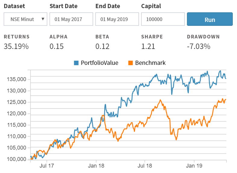
For more details, we can go and run the full backtest.

More technical strategies¶

The strategy above is quite general for implementing any technical indicator based strategy. As we see the core logic is implemented in the signal_function. By simply altering this function we can create a range of different strategies with different indicators or combination of them. For more examples of such strategies please visit our demo page on Github.

This is a useful place with good introductory materials on different indicators ↩
See This for more details ↩