Factor Based Strategies on Blueshift®¶

What is a factor¶

Market theories¹ tell us that returns of any stock can be explained by a set of hidden variables, plus a residual bit unique to that stock. Usually, we take overall market returns as the sole explainer. In this world, the value investor's job is to find stocks with high expected residual returns, assuming valuation measures can capture it. It turns out parts of this residual can be further explained by other fundamental characteristics of the stock. If they are stable and consistent, each of such characteristics can be thought of as a risk factor. In such a world, an investor's job is to identify factors with high expected returns and design portfolios to capture them. This is, in a nutshell, the essence of factor investing. We systematically probe the drivers of the markets, instead of taking concentrated exposure on idiosyncratic risks.

The maths of factor models¶

The Capital Asset Pricing Model¹ tells us the expected returns of a stock can be expressed as

$\mathop{\mathbb{E}}R=R_{f}+\beta(\mathop{\mathbb{E}}R_{M} - R_{f})$

Here $\mathop{\mathbb{E}}$ is the expectation operator, $R$ the stock returns, $R_{f}$ the risk-free return, $R_{M}$ the returns of the market portfolio, and $\beta$ is the sensitivity of $R$ to $R_{M}$ . The realized returns under this model is then

$R = \alpha + \beta(R_{M} - R_{f})+\epsilon$

Here $\alpha$ is the returns not explained by the market factors and $\epsilon$ is a zero-mean stock specific innovation (also known as idiosyncratic risk). All factor models extend this basic equations ( expected and realized returns) respectively as below

$\mathop{\mathbb{E}}R=R_{f}+\sum_{k=1}^N\beta_{k}(\mathop{\mathbb{E}}\Delta F_{k})$

$R = \alpha_{F} + \sum_{k=1}^N\beta_{k}(\Delta F_{k})+\epsilon_{F}$

These are with similar interpretation. The $\alpha_{F}$ and $\epsilon_{F}$ are same as $\alpha$ and $\epsilon$ as above, accounting for the extra factors (in addition to the market factor $R_{M}-R_{f}$ ). $\Delta F_{k}$ is the realized change in the factor, and $\mathop{\mathbb{E}}\Delta F_{k}$ is the expected change, also known as the risk premium. $beta_{k}$ is the sensitivity (loading) of the asset to the particular factor $k$ .

The objective of all factor models is to find a set of factors $F_{k}$ s such that the factor sensitivity as well as the risk premia are stable and predictable. Such strategies, when properly designed, can extract the returns (as a result of exposure to the factors risk) over and above the market returns. Most of factor research revolves how to find, evaluate and verify such factors, and how to build portfolios to control exposure to a particular factor or a set of factors.

The cross-sectional momentum factor¶

Factor investing is an active area of investment research. Apart from the market factor, there are many other factors proposed in many research papers since Fama and French ² first came up with their three factor model. One such time-tested factor is the cross-sectional momentum factor, first scrutinized by Jegadeesh and Titman ³. The strategy is as follows:

Rank all assets in the universe based on their past returns.
Buy the top x-percentile and sell the bottom x-percentile (even if they are going up in prices).
Rebalance after a specified holding period

The past returns are typically computed for 1 year, one month prior to rebalance. Holding period is typically one month. It is also common to apply a liquidity filter to the asset universe to weed out illiquid stocks which may skew the factor exposure.

Creating a custom pipeline package¶

If you have gone through the previous section, this strategy looks like a perfect fit for using pipeline. We are first going to create a custom pipeline package just like we did in our technical indicator tutorials. As usual, we create a directory at the root of our workspace named pipelines, and inside that directory create a source file (using any template, we will be deleting all template codes) named pipelines. Copy the code from here and paste it in the new source file, overwriting all existing contents. Save and go back to our workspace. Our custom pipeline library is ready!

The factor computation¶

If we take a look at the file we just created, we will find a function called period_returns. This is the function that computes our factor. The function looks like below:

def period_returns(lookback):
    class SignalPeriodReturns(CustomFactor):
        inputs = [EquityPricing.close]
        def compute(self,today,assets,out,close_price):
            start_price = close_price[0]
            end_price = close_price[-1]
            returns = end_price/start_price - 1
            out[:] = returns
    return SignalPeriodReturns(window_length = lookback)

We have already seen example of customizing factors and filters. Here again we overwrite the compute function. The only input is close price. We simply calculate the returns over the periods and assign it to our out variable. Another filter function we will use is a volume filter, which we have already seen before once.

Implementing the strategy¶

Let's now create a new source anywhere in our workspace from one of the Buy and Hold templates. Let's add the following line to the top before all imports, to import the functions we need from our custom library we just created.

from blueshift_library.pipelines.pipelines import average_volume_filter, period_returns
from blueshift.errors import NoFurtherDataError

We also import a special exception NoFurtherDataError so that we can catch when there are no data to be fed to the pipeline. Let's now define the initialize function as below:

def initialize(context):
    context.params = {'lookback':12,
                      'percentile':0.05,
                      'min_volume':1E7
                      }

    # Call rebalance function on the first trading day of each month
    schedule_function(strategy, date_rules.month_start(), 
            time_rules.market_close(minutes=1))

    # Set up the pipe-lines for strategies
    attach_pipeline(make_strategy_pipeline(context), 
            name='strategy_pipeline')

Here we define the parameters of our strategy, the lookback for our returns computation (12 months), volume filter (dollar volume greater than 10 million) and percentile to group stocks to buy or sell (as we shall see later). Then we schedule a function called strategy to be called every month (matching the holding period). Finally we build a pipeline in a function called make_strategy_pipeline (to be defined later) and attach to our strategy.

Building the pipeline¶

The pipeline building looks like below:

def make_strategy_pipeline(context):
    pipe = Pipeline()

    # get the strategy parameters
    lookback = context.params['lookback']*21
    v = context.params['min_volume']

    # Set the volume filter
    volume_filter = average_volume_filter(lookback, v)

    # compute past returns
    momentum = period_returns(lookback)
    pipe.add(momentum,'momentum')
    pipe.set_screen(volume_filter)

    return pipe

Here as usual we instantiate an empty pipeline, call upon or filter ( volume_filter) and factor (momentum) using our library functions we just created, add the factor under a column (also named momentum), and set the screen with the filter. Note, here we multiply the lookback with 21, to convert from months to days.

Running the strategy¶

The main strategy function we scheduled is very simple:

def strategy(context, data):
    generate_signals(context, data)
    rebalance(context,data)

This computes the factors and do the rebalancing at the set intervel.

Computing the factors¶

This is done in the generate_signals function that looks like below:

def generate_signals(context, data):
    try:
        pipeline_results = pipeline_output('strategy_pipeline')
    except NoFurtherDataError:
        context.long_securities = []
        context.short_securities = []
        return

    p = context.params['percentile']
    momentum = pipeline_results.dropna().sort_values('momentum')
    n = int(len(momentum)*p)

    if n == 0:
        print("{}, no signals".format(data.current_dt))
        context.long_securities = []
        context.short_securities = []

    context.long_securities = momentum.index[-n:]
    context.short_securities = momentum.index[:n]

This is the heart of the implementation. Here we query the pipeline (see here) which computes the result and return it in the array pipeline_results. We sort this array (remember this array is indexed by the assets) by the factor column we want (momentum in this case). We pick up the top p percentile of stocks to buy (storing it in context.long_securities) and bottom p percentile to short (context.short_securities). This is the classic cross-sectional momentum strategy. Note, by design, we always have same number of stocks to buy and sell, giving us a market neutral portfolio.

Carrying out the rebalancing¶

Finally we trade the securities in our long and short list in the rebalance function:

from blueshift.api import order_target_percent

def rebalance(context,data):
    # weighing function
    n = len(context.long_securities)
    if n < 1:
        return

    weight = 0.5/n

    # square off old positions if any
    for security in context.portfolio.positions:
        if security not in context.long_securities and \
           security not in context.short_securities:
               order_target_percent(security, 0)

    # Place orders for the new portfolio
    for security in context.long_securities:
        order_target_percent(security, weight)
    for security in context.short_securities:
        order_target_percent(security, -weight)

This function defines a base weight. Then it first check if we have open positions in any stocks that are NOT in our current long or short lists and close them out. We do that by querying the special variable context. Then it loops through our long and short lists and place new orders with the target weight with sign.

Running a quick backtest¶

Now that our strategy is done, let's hit the quick run button, selecting NSE daily as our dataset and date range as 1^st May 2010 to 25^th July 2019 and capital at 100,000. The result looks like below:

result

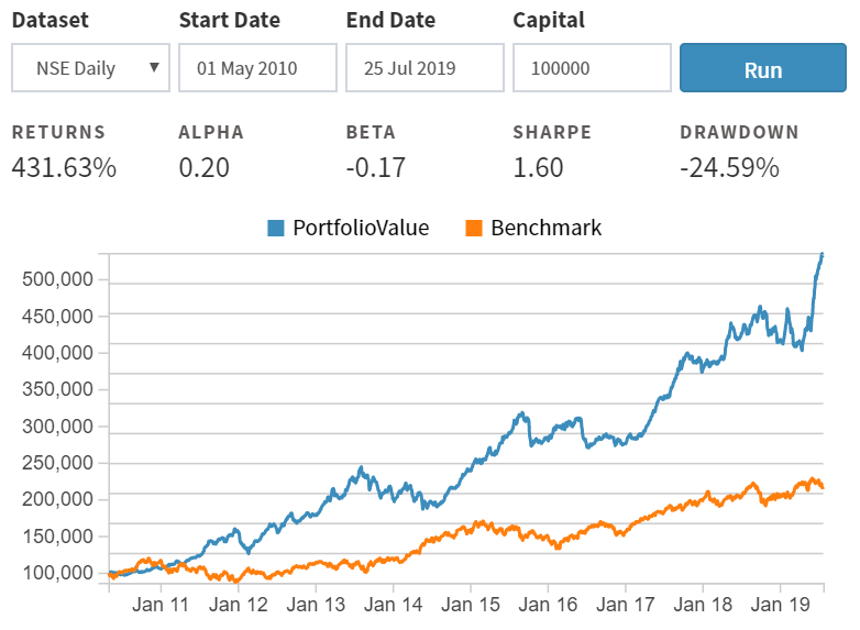
For more details, we can go and run the full backtest.

More factor strategies¶

Any factor based strategy can be implemented using the above guidelines. We have to first define a factor function (like period_returns above) and then can use the rest of the strategy code to implement it. This function can be anything, as long as it returns a single numerical value for each stocks. We rank our stocks based on that value, choose a long/short portfolio based on this rankings and carry out the trades. For more examples of such strategies please visit our demo page on Github. For a list of factor based strategies in equity markets see here.

See here for an introduction to the Capital Asset Pricing Model. ↩↩
See here for an introduction to the three factor model. ↩
See here for the original research paper. ↩