Getting Started with Notebooks on Blueshift

We first start by importing a few required functions from the blueshift.research module. The methods list_datasets and use_dataset allow us to list available datasets and select one, respectively as shown below:

from blueshift.research import list_datasets, use_dataset
print(list_datasets())

['nse']

We also import the symbol, current and history functions from the blueshift.research module. These form the primary interface to query the selected dataset. Note, we must call ``use_dataset`` before we can use any of these three functions.

from blueshift.research import symbol, current, history
# This is going to take some time!!!
use_dataset('nse')

Once a dataset is selected, we can use the symbol function to fetch an asset from the dataset selected using a string ticker (as we do while writing strategy code). Also, similar to strategy code, we can use the current and history method to fetch data. The signatures of these functions are as show below:

• symbol(sym, dt=None, *args, **kwargs): Returns the asset corresponding to the ticker sym. Specify dt (a pandas Timestamp) to fix the asset resolution time. See symbol for more details. Returns an `asset <>`__ object

• current(assets, columns=’close’, dt=None, last_known=True): Returns the current value of the asset(s) for the chosen column(s). Specifiy dt (a pandas Timestamp) to select the query time (defaults to current timestamp). Set last_known to False to return a NaN value in case no data avaiable that matches the exact time specified. The return type depends on the input values. See current for more details

• history(assets, columns, nbars, frequency, dt=None, adjusted=True): Returns the historical data for the asset(s) and column(s). The meaning of dt is same as in current above. Set adjusted to False if no adjustments is to be applied. The return type depends on the input values. See history for more details

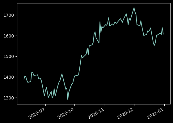
Since we have already selected the dataset in the above, we can now use these functions to fetch data and make some plots!

import matplotlib.pyplot as plt

plt.style.use('dark_background')

asset = symbol('ACC')
px = history(asset, ['close'], 100, '1d', dt='2023-06-30')
px.close.plot()

<Axes: >

Let’s create a slightly better looking plot, using the plotly library

import plotly.graph_objects as go

fig = go.Figure([go.Scatter(x=px.index, y=px.close)])
fig.update_layout(template='plotly_dark')
fig.show()

Now that you know how to fetch assets and data, you are ready to explore your ideas. For a list of available packages, see whitelist.